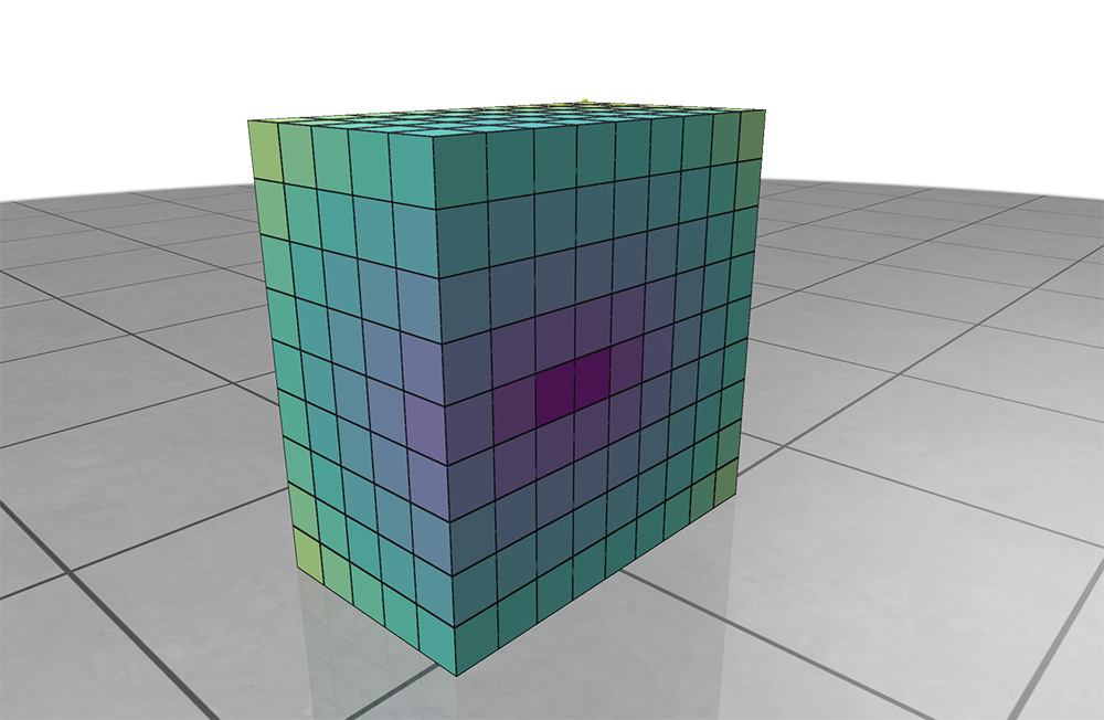
Scalar Quantities
Visualize scalar-valued data at the nodes or cells of a volume grid.
Example: registering a volume grid and adding a scalar quantity
import polyscope as ps
import numpy as np

ps.init()

# define the resolution and bounds of the grid
dims = (20, 20, 20)
bound_low = (-3., -3., -3.)
bound_high = (3., 3., 3.)

# register the grid
ps_grid = ps.register_volume_grid("sample grid", dims, bound_low, bound_high)

# your dimX*dimY*dimZ buffer of data
scalar_vals = np.zeros(dims[0], dims[1], dims[2])

# add a scalar function on the grid
ps_grid.add_scalar_quantity("node scalar", scalar_vals, defined_on='nodes')

# set some scalar options
ps_grid.add_scalar_quantity("node scalar2", scalar_vals, defined_on='nodes',
                            vminmax=(-5., 5.), cmap='blues', enabled=True)

ps.show()
Add scalars
VolumeGrid.add_scalar_quantity(name, values, defined_on='nodes', datatype="standard", **scalar_args)
Add a scalar quantity defined at the nodes of the grid.
namestring, a name for the quantityvaluesa numpy array of shape(dimX, dimY, dimZ)giving scalars at nodes/cells.defined_onone of'nodes', 'cells', is this data a value per node or a value per cell?
This function also accepts optional keyword arguments listed below, which customize the appearance and behavior of the quantity.
Add implicit scalars
Implicit helpers
Implicit helpers offer an easier way to interface your data with Polyscope. You define a callback function which can be called at a batch of xyz coordinates to return a batch of values, and pass that function as input. Polyscope then automatically takes care of calling the function at the appropriate locations to sample the function onto the grid.
See Implicit Helpers for more details about implicit helpers.
VolumeGrid.add_scalar_quantity_from_callable(name, func, defined_on='nodes', datatype="standard", **scalar_args)
Add a scalar quantity defined at the nodes of the grid, sampling automatically via a callable function.
funcis a function which performs a batch of evaluations of the implicit function. It should take a(Q,3)numpy array of world-space xyz locations at which to evaluate the function whereQis the number of queries, and return a(Q,)numpy array of results.
This function also accepts optional keyword arguments listed below, which customize the appearance and behavior of the quantity.
Categorical Scalars
Scalar quantities can also be used to visualize integer-valued labels such as categories, classes, segmentations, flags, etc.
Add the labels as a scalar quantity where the values just happen to be integers (each integer represents a particular class or label), and set datatype='categorical'. This will change the visualization to a different set of defaults, adjust some shading rules, and use a distinct color from the colormap for each label.
Color Bars
Each scalar quantity has an associated color map, which linearly maps scalar values to a spectrum of colors for visualization.
See colormaps for a listing of the available maps, and use add_scalar_quantity(..., cmap="cmap_name") to choose the map.
The colormap is always displayed with an inline colorbar in the structures panel, which also gives a histogram of the scalar values in your quantity.
The limits (vminmax) of the colormap range are given by the two numeric fields below the colored display. You can click and drag horizontally on these fields to adjust the map range, or ctrl-click (cmd-click) to enter arbitrary custom values.
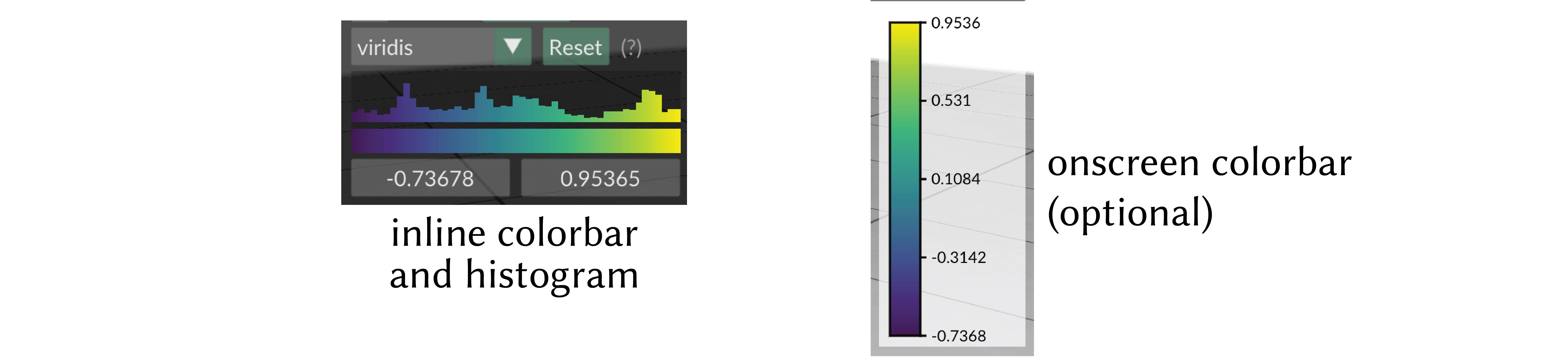
onscreen colorbar
Optionally an additional onscreen colorbar, which is more similar to the colorbars used in other plotting libraries, can be enabled with add_scalar_quantity(..., onscreen_colorbar_enabled=True).
By default it is positioned automatically inline with the other UI elements, or it can be manually positioned with add_scalar_quantity(..., onscreen_colorbar_location=(400., 400.)).
You can even export this color map to an .svg file for creating figures via the options menu.
Scalar Quantity Options
When adding a scalar quantity, the following keyword options can be set. These are available for all kinds of scalar quantities on all structures.
Keyword arguments:
enabledboolean, whether the quantity is initially enabled (note that generally only one quantitiy can be shown at a time; the most recent will be used)datatype, one of"standard","symmetric","magnitude", or"categorical", affects default colormap and map range, and the categorical policies mentioned abovevminmax, a 2-tuple of floats, specifying the min and max range for colormap limits; the default isNone, which computes the min and max of the data- colormap keywords:
cmap, which colormap to useonscreen_colorbar_enabledset toTrueto enable an additional traditional colormaponscreen_colorbar_locationset to screen coordinates like(400., 400.)to position the onscreen colorbar manually (default is automatic)
- isoline keywords (darker-shaded stripes showing isocontours of the scalar field):
isolines_enabledare isolines enabled (default:False)isoline_styleone ofstripe,'contour(default:stripe)isoline_periodhow wide should the darkend stripes be, in data units (default: dynamically estimated)isoline_period_relativeif true, interpret the width value as relative to the world coordinate length scale (default:False)isoline_darknesshow much darker should the alternating stripes be (default:0.7)isoline_contour_thicknesshow thick should the contour lines be (default:0.3)
If not specified, these optional parameters will assume a reasonable default value, or a persistent value if previously set.
Visualizing Isosurfaces
For a scalar values at nodes, we can additionally extract isosurfaces (aka levelsets) via the marching cubes algorithm, and visualize them as surface meshes.
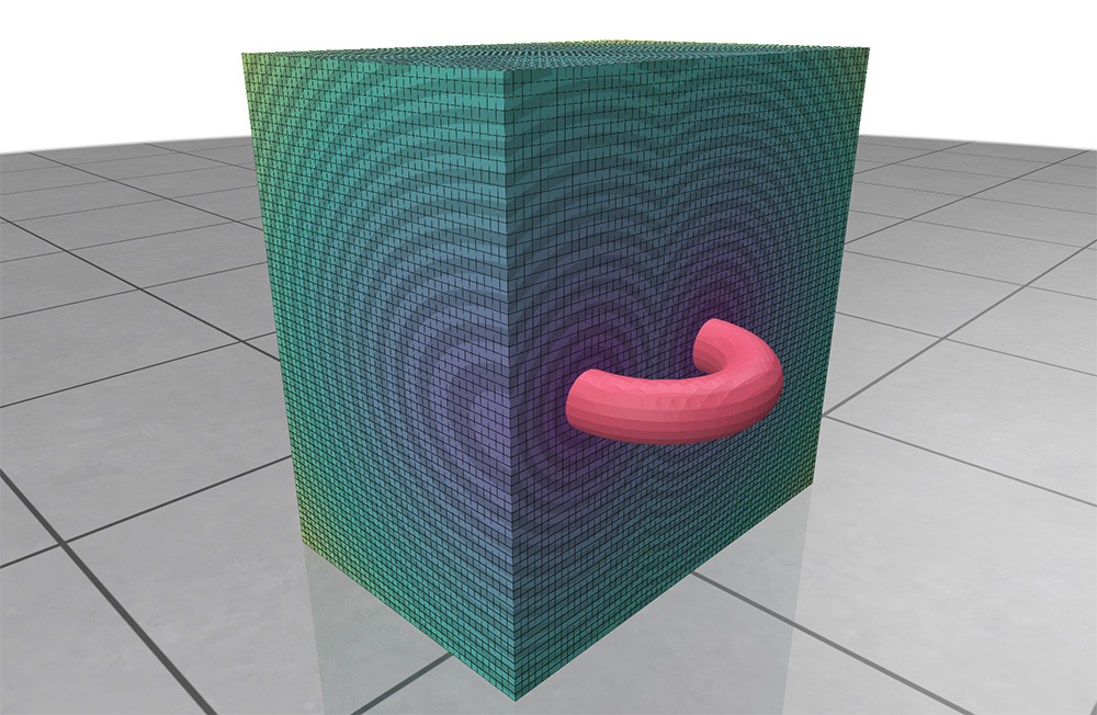
Example: visualizing scalar isosurfaces
# continued after the grid as been set up as in the example above

# draw the isosurfce, hiding the usual grid so it is visible
ps_grid.add_scalar_quantity("node scalar", scalar_vals, defined_on='nodes',
                            enable_isosurface_viz=True, isosurface_level=0.5,
                            isosurface_color=(0.2, 0.1, 0.8),
                            enable_gridcube_viz=False)
ps.show()

# draw the isosurface, using a slice plane to cut through it
ps_grid.add_scalar_quantity("node scalar", scalar_vals, defined_on='nodes',
                            enable_isosurface_viz=True, isosurface_level=0.5,
                            slice_planes_affect_isosurface=False)
ps.add_scene_slice_plane()
ps.show()


# extract the isosurface as its own mesh structure
scalarQ->registerIsosurfaceAsMesh("my isosurface mesh");
ps_grid.add_scalar_quantity("node scalar", scalar_vals, defined_on='nodes',
                            enable_isosurface_viz=True, isosurface_level=0.5,
                            register_isosurface_as_mesh_with_name='isosurface mesh')
The following optional arguments to the node scalar quantity adder affect the behavior of isosurfaces.
Note
By default, the grid obscures the isosurface so it cannot be seen. You probably want to either:
- use a slice plane, along with the
slice_planes_affect_isosurface=Falseoption, or - use
enable_gridcube_viz=Falseto disable the default grid visualization
enable_gridcube_vizboolean, is the usual grid cube visualization drawnenable_isosurface_vizboolean, should the isosurface be extracted and drawnisosurface_levelfloat, which isolevel should be extractedisosurface_color3-tuple of floats, color of the isosurface meshslice_planes_affect_isosurfaceboolean, do slice planes affect the isosurfaceregister_isosurface_as_mesh_with_namestring, if given, register the isosurface as a new mesh with this name. Passing""generates a default name.